The SHARPy Case files
SHARPy takes as input a series of .h5 files that contain the numerical data and a .sharpy file that contains
the settings for each of the solvers. How these files are generated is at the user’s discretion, though templates are
provided, and all methods are valid as long as the required variables are provided with the appropriate format.
Modular Framework
SHARPy is built with a modular framework in mind. The following diagram shows the strutuctre of a nonlinear, time marching aeroelastic simulation
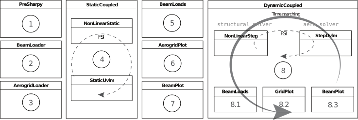
Each of the blocks correspond to individual solvers with specific settings. How we choose which solvers to run, in which order and with what settings is done through the solver configuration file, explained in the next section.
Solver configuration file
The solver configuration file is the main input to SHARPy. It is a ConfigObj
formatted file with the .sharpy extension. It contains the settings for each of the solvers and the order in which
to run them.
A typical way to assemble the solver configuration file is to place all your desired settings
in a dictionary and then convert to and write your ConfigObj. If a setting is not provided the default value will be used. The settings that each solver takes, its type and default value are explained in their relevant documentation pages.
import configobj
filename = '<case_route>/<case_name>.sharpy'
config = configobj.ConfigObj()
config.filename = filename
config['SHARPy'] = {'case': '<your SHARPy case name>',  # an example setting
                    # Rest of your settings for the PreSHARPy class
                    }
config['BeamLoader'] = {'orientation': [1., 0., 0.],  # an example setting
                        # Rest of settings for the BeamLoader solver
                        }
# Continue as above for the remainder of solvers that you would like to include

# finally, write the config file
config.write()
The resulting .sharpy file is a plain text file with your specified settings for each of
the solvers.
Note that, therefore, if one of your settings is a np.array, it will get transformed into
a string of plain text before being read by SHARPy. However, any setting with list(float) specified as its setting type will get converted into a np.array once it is read by SHARPy.
FEM file
The case.fem.h5 file has several components. We go one by one:
num_node_elem [int]: number of nodes per element.Always 3 in our case (3 nodes per structural elements - quadratic beam elements).
num_elem [int]: number of structural elements.num_node [int]: number of nodes.For simple structures, it is
num_elem*(num_node_elem - 1) - 1. For more complicated ones, you need to calculate it properly.coordinates [num_node, 3]: coordinates of the nodes in body-attached FoR (A).connectivites [num_elem, num_node_elem]: Beam element’s connectivities.Every row refers to an element, and the three integers in that row are the indices of the three nodes belonging to that elem. Now, the catch: the ordering is not as you’d think. Order them as
[0, 2, 1]. That means, first one, last one, central one. The following image shows the node indices inside the circles representing the nodes, the element indices in blue and the resulting connectivities matrix next to it. Connectivities are tricky when considering complex configurations. Pay attention at the beginning and you’ll save yourself a lot of trouble.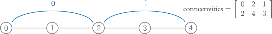
stiffness_db [:, 6, 6]: database of stiffness matrices.The first dimension has as many elements as different stiffness matrices are in the model.
elem_stiffness [num_elem]: array of indices (starting at 0).It links every element (index) to the stiffness matrix index in
stiffness_db. For exampleelem_stiffness[0] = 0;elem_stiffness[2] = 1means that the element0has a stiffness matrix equal tostiffness_db[0, :, :], and the second element has a stiffness matrix equal tostiffness_db[1, :, :].The shape of a stiffness matrix, \(\mathrm{S}\) is:
\[\begin{split}\mathrm{S} = \begin{bmatrix} EA & & & & & \\ & GA_y & & & & \\ & & GA_z & & & \\ & & & GJ & & \\ & & & & EI_y & \\ & & & & & EI_z \\ \end{bmatrix}\end{split}\]with the cross terms added if needed.
mass_dbandelem_massfollow the same scheme than the stiffness, but the mass matrix is given by:\[\begin{split}\mathrm{M} = \begin{bmatrix} m\mathbf{I} & -\tilde{\boldsymbol{\xi}}_{cg}m \\ \tilde{\boldsymbol{\xi}}_{cg}m & \mathbf{J}\\ \end{bmatrix}\end{split}\]where \(m\) is the distributed mass per unit length \(kg/m\) , \((\tilde{\bullet})\) is the skew-symmetric matrix of a vector and \(\boldsymbol{\xi}_{cg}\) is the location of the centre of gravity with respect to the elastic axis in MATERIAL (local) FoR. And what is the Material FoR? This is an important point, because all the inputs that move WITH the beam are in material FoR. For example: follower forces, stiffness, mass, lumped masses…
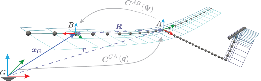
The material frame of reference is noted as \(B\). Essentially, the \(x\) component is tangent to the beam in the increasing node ordering, \(z\) looks up generally and \(y\) is oriented such that the FoR is right handed.
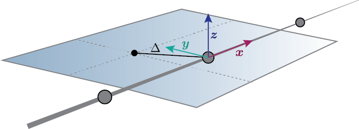
In the practice (vertical surfaces, structural twist effects…) it is more complicated than this. The only sure thing about \(B\) is that its \(x\) direction is tangent to the beam in the increasing node number direction. However, with just this, we have an infinite number of potential reference frames, with \(y\) and \(z\) being normal to \(x\) but rotating around it. The solution is to indicate a
for_delta, or frame of reference delta vector (\(\Delta\)).
Now we can define unequivocally the material frame of reference. With \(x_B\) and \(\Delta\) defining a plane, \(y_b\) is chosen such that the \(z\) component is oriented upwards with respect to the lifting surface.
From this definition comes the only constraint to \(\Delta\): it cannot be parallel to \(x_B\).
frame_of_reference_delta [num_elem, num_node_elem, 3]: rotation vector to FoR \(B\).contains the \(\Delta\) vector in body-attached (\(A\)) frame of reference.
As a rule of thumb:
\[\begin{split}\Delta = \begin{cases} [-1, 0, 0], \quad \text{if right wing} \\ [1, 0, 0], \quad \text{if left wing} \\ [0, 1, 0], \quad \text{if fuselage} \\ [-1, 0, 0], \quad \text{if vertical fin} \\ \end{cases}\end{split}\]These rules of thumb only work if the nodes increase towards the tip of the surfaces (and the tail in the case of the fuselage).
structural_twist [num_elem, num_node_elem]: Element twist.Technically not necessary, as the same effect can be achieved with
FoR_delta.boundary_conditions [num_node]: boundary conditions.An array of integers
(np.zeros((num_node, ), dtype=int))and contains all0except forOne node NEEDS to have a
1, this is the reference node. Usually, the first node has 1 and is located in[0, 0, 0]. This makes things much easier.If the node is a tip of a beam (is not attached to 2 elements, but just 1), it needs to have a
-1.
beam_number [num_elem]: beam index.Is another array of integers. Usually you don’t need to modify its value. Leave it at 0.
app_forces [num_elem, 6]: applied forces and moments.Contains the applied forces
app_forces[:, 0:3]and momentsapp_forces[:, 3:6]in a given node.Important points: the forces are given in Material FoR (check above). That means that in a symmetrical model, a thrust force oriented upstream would have the shape
[0, T, 0, 0, 0, 0]in the right wing, while the left would be[0, -T, 0, 0, 0, 0]. Likewise, a torsional moment for twisting the wing leading edge up would be[0, 0, 0, M, 0, 0]for the right, and[0, 0, 0, -M, 0, 0]for the left. But careful, because an out-of-plane bending moment (wing tip up) has the same sign (think about it).lumped_mass [:]: lumped masses.Is an array with as many masses as needed (in kg this time). Their order is important, as more information is required to implement them in a model.
lumped_mass_nodes [:]: Lumped mass nodes.Is an array of integers. It contains the index of the nodes related to the masses given in lumped_mass in order.
lumped_mass_inertia [:, 3, 3]: Lumped mass inertia.Is an array of
3x3inertial tensors. The relationship is set by the ordering as well.lumped_mass_position [:, 3]: Lumped mass position.Is the relative position of the lumped mass with respect to the node (given in
lumped_masss_nodes) coordinates. ATTENTION: the lumped mass is solidly attached to the node, and thus, its position is given in Material FoR.


Aerodynamics file
All the aerodynamic data is contained in case.aero.h5.
It is important to know that the input for aero is usually based on elements (and inside the elements, their nodes). This causes sometimes an overlap in information, as some nodes are shared by two adjacent elements (like in the connectivities graph in the previous section). The easier way of dealing with this is to make sure the data is consistent, so that the properties of the last node of the first element are the same than the first node of the second element.
Item by item:
airfoils: Airfoil group.In the
aero.h5file, there is a Group calledairfoils. The airfoils are stored in this group (which acts as a folder) as a two-column matrix with \(x/c\) and \(y/c\) in each column. They are named'0', '1', and so on.chords [num_elem, num_node_elem]: ChordIs an array with the chords of every airfoil given in an element/node basis.
twist [num_elem, num_node_elem]: Twist.Has the twist angle in radians. It is implemented as a rotation around the local \(x\) axis.
sweep [num_elem, num_node_elem]: Sweep.Same here, just a rotation around \(z\).
airfoil_distribution [num_elem, num_node_elem]: Airfoil distribution.Contains the indices of the airfoils that you put previously in
airfoils.surface_distribution [num_elem]: Surface integer array.It contains the index of the surface the element belongs to. Surfaces need to be continuous, so please note that if your beam numbering is not continuous, you need to make a surface per continuous section.
surface_m [num_surfaces]: Chordwise panelling.Is an integer array with the number of chordwise panels for every surface.
m_distribution [string]: Discretisation method.Is a string with the chordwise panel distribution. In almost all cases, leave it at
uniform.aero_node [num_node]: Aerodynamic node definition.Is a boolean (
TrueorFalse) array that indicates if that node has a lifting surface attached to it.elastic_axis [num_elem, num_node_elem]: elastic axis.Indicates the elastic axis location with respect to the leading edge as a fraction of the chord of that rib. Note that the elastic axis is already determined, as the beam is fixed now, so this settings controls the location of the lifting surface wrt the beam.
control_surface [num_elem, num_node_elem]: Control surface.Is an integer array containing
-1if that section has no control surface associated to it, and0, 1, 2 ...if the section belongs to the control surface0, 1, 2 ...respectively.control_surface_type [num_control_surface]: Control Surface type.Contains
0if the control surface deflection is static, and1is it is dynamic.control_surface_chord [num_control_surface]: Control surface chord.Is an INTEGER array with the number of panels belonging to the control surface. For example, if
M = 4and you want your control surface to be \(0.25c\), you need to put1.control_surface_hinge_coord [num_control_surface]: Control surface hinge coordinate.Only necessary for lifting surfaces that are deflected as a whole, like some horizontal tails in some aircraft. Leave it at
0if you are not modelling this.airfoil_efficiency [num_elem, num_node_elem, 2, 3]: Airfoil efficiency.This is an optional setting that introduces a user-defined efficiency and constant terms to the mapping between the aerodynamic forces calculated at the lattice grid and the structural nodes. The formatting of the 4-dimensional array is simple. The first two dimensions correspond to the element index and the local node index. The third index is whether the term is the multiplier to the force
0or a constant term1. The final term refers to, in the local, body-attachedBframe, the factors and constant terms for:fy, fz, mx. For more information on how these factors are included in the mapping terms seesharpy.aero.utils.mapping.aero2struct_force_mapping().polarsGroup (optional): Use airfoil polars to correct aerodynamic forces.This is an optional group to add if correcting the aerodynamic forces using airfoil polars is desired. A polar should be included for each airfoil defined. Each entry consists of a 4-column table. The first column corresponds to the angle of attack (in radians) and then the
C_L,C_DandC_M.
Multibody file
All the aerodynamic data is contained in case.mb.h5.
This file encapsulates both the initial conditions for the multiple bodies, and the constraints between them.
Item by item:
num_bodies: Number of bodies.num_constraints: Number of constraints between bodies.The initial conditions for each body and the constraint definitions are defined in groups. The body groups are named as
body_xx, where the xx is replaced with a two digit body number starting from 00, e.g.body_00. Each of these groups should have the following items:FoR_acceleration [6]: Frame of reference initial acceleration.An array of the stacked linear and rotational initial accelerations in the inertial frame.
FoR_velocity [6]: Frame of reference initial velocity.An array of the stacked linear and rotational initial velocities in the inertial frame.
FoR_position [6]: Frame of reference initial position.An array of the stacked linear and rotational initial positions in the inertial frame.
quat [4]: Frame of reference initial orientation.A quaternion describing the initial rotation between the body attached and inertial frames.
body_number: Body number.An integer used to identify the body when creating constraints.
FoR_movement: Type of frame of reference movement.Use “free” to include rigid body motion, or “prescribed” for a clamped body.
The constraint groups are named similarly to the bodies, using constraint_xx where xx is the two digit constraint number
starting from 00. Each of these groups should have the following items:
scalingFactor: Scaling factor.This value scales the multibody equations, where generally settings to
dt^2provides acceptable results.behaviour: Constraint behaviour.This string defines the type of constraint applied to a single or multiple bodies. A wide range of standard lower-pair kinematic joints are available, such as hinge and spherical joints, as well as prescribed rotation joints. A list of the available joints can be found in
sharpy/structure/utils/lagrangeconstraints.pyandsharpy/structure/utils/lagrangeconstraintsjax.py, depending on the solver being used. Due to every constraint being different, further parameters depend upon the constraint type used. These parameters are added as variables to the constraint group. Some examples which may be included are listed below:body_FoR: Body frame of reference number.The number of the body which is constrained by its body attached frame of reference. For example for a double pendulum, this would be the lower link.
body: Body number.The number of the body which is constrained by one of its nodes. For example for a double pendulum, this would be the upper link.
node_in_body: Node in body.This is paired to the
bodyparameter, and this indicates which node within the body is to be constrained.rot_axisB [3]: Rotation axis in the B frame.For a hinge constraint, this defines a vector for the hinge axis for the
body. This is defined in the material frame.rot_axisA2 [3]: Rotation axis in the A frame.For a hinge constraint, this defines a vector for the hinge axis for the
body_FoR. This is defined in the body attached frame.controller_id: Controller ID for using an actuated constraint.This should use the same ID as the
MultibodyControllerused in theDynamicCoupledsimulation, allowing the rotation to be controlled over time.aerogrid_warp_factor [num_elem, 3]: Aerodynamic grid warping factor.For simulating wings with dynamic sweep by a local rotation around the z axis, the aerodynamic grid needs to warp to account for this. To create a smooth warp, it can be preferred to gradually change the sweep (and therefore chord to maintain the “same” geometry) at elements around the discontinuity. This parameter sets the sweep per node using this parameter to scale the input angle. If not included, it will be ignored when generating the aerodynamic grid and have no effect.
Nonlifting Body file
All the nonlifting body data is contained in case.nonlifting_body.h5.
The idea behind the structure of the model definition of nonlifting bodies in SHARPy is similiar to the aerodynamic one for lifting surfaces. Again for each node or element we define several parameters.
Item by item:
shape: Type of geometrical form of 3D nonlifting body.In the
nonlifting_body.h5file, there is a Group calledshape. The shape indicates the geometrical form of the nonlifting body. Common options for this parameter are'cylindrical'and'specific'. For the former, SHARPy expects rotational symmetric cross-section for which only a radius is required for each node. For the'specific'option, SHARPy can create a more unique nonlifting body geometry by creating an ellipse at each fuselage defined by \(\frac{y^2}{a^2}+\frac{z^2}{b^2}=1\) with the given ellipse axis lengths \(a\) and \(b\). Further, SHARPy lets define the user to create a vertical offset from the node with \(z_0\).radius [num_node]: Cross-sectional radius.Is an array with the radius of specified for each fuselage node.
a_ellipse [num_node]: Elliptical axis lengths along the local y-axis.Is an array with the length of the elliptical axis along the y-axis.
b_ellipse [num_node]: Elliptical axis lengths along the local z-axis.Is an array with the length of the elliptical axis along the z-axis.
z_0_ellipse [num_node]: Vertical offset of the ellipse center from the beam node.Is an array with the vertical offset of the center of the elliptical cross-section from the fuselage node.
surface_m [num_surfaces]: Radial panelling.Is an integer array with the number of radial panels for every surface.
nonlifting_body_node [num_node]: Nonlifting body node definition.Is a boolean (
TrueorFalse) array that indicates if that node has a nonlifting body attached to it.surface_distribution [num_elem]: Nonlifting Surface integer array.It contains the index of the surface the element belongs to. Surfaces need to be continuous, so please note that if your beam numbering is not continuous, you need to make a surface per continuous section.
Time-varying force input file (.dyn.h5)
The .dyn.h5 file is an optional input file that may contain force and acceleration inputs that vary with time.
This is intended for use in dynamic problems. For SHARPy to look for and use this file the setting unsteady in the
BeamLoader must be turned to on.
Appropriate data entries in the .dyn.h5 include:
dynamic_forces [num_t_steps, num_node, 6]: Dynamic forces in body attachedBframe.Forces given at each time step, for each node and then for the 6 degrees of freedom (
fx, fy, fz, mx, my, mz) in a body-attached (local) frame of referenceB.for_pos [num_t_steps, 6]: Body frame of reference (A FoR) position.Position of the reference frame A in time.
for_vel [num_t_steps, 6]: Body frame of reference (A FoR) velocity.Velocity of the reference frame A in time.
for_acc [num_t_steps, 6]: Body frame of reference (A FoR) acceleration.Acceleration of the reference frame A in time.
If a case is restarted from a pickle file, the .dyn.h5 file should include the dynamic information for the previous simulation (that will be discarded) and the information for the new simulation.