A first test case with SHARPy
This notebook explains how to create a prismatic cantilever and flexible wing in SHARPy. It aims to provide a big picture about the simulations available in SHARPy describing the very fundamental concepts.
This notebook requires around two hours to be completed.
Generation of the aeroelastic model
This section explains how to generate the input files for SHARPy including the structure, the aerodynamics and the simulation details.
[3]:
# Loading of the used packages
import numpy as np              # basic mathematical and array functions
import os                       # Functions related to the operating system
import matplotlib.pyplot as plt # Plotting library

import sharpy.sharpy_main                  # Run SHARPy inside jupyter notebooks
import sharpy.utils.plotutils as pu        # Plotting utilities
from sharpy.utils.constants import deg2rad # Constant to conver degrees to radians

import sharpy.utils.generate_cases as gc
The generate cases module of SHARPy includes a number of templates for the creation of simple cases using common parameters as inputs. It also removes clutter from this notebook.
The following cell configures the plotting library to show the next graphics, it is not part of SHARPy.
[4]:
%%capture
! pip install plotly
Define the problem parameters
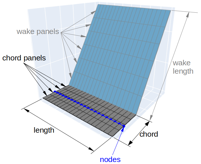
In this section, we define the basic parameters to generate a model for the wing shown in the image below. We use SI units for all variables.
[5]:
%config InlineBackend.figure_format = 'svg'
from IPython.display import Image
url = ('https://raw.githubusercontent.com/ImperialCollegeLondon/sharpy/dev_example/docs/' +
       'source/content/example_notebooks/images/simple_wing_scheme.png')
Image(url=url, width=800)
[5]:
[6]:
# Geometry
chord = 1.         # Chord of the wing
aspect_ratio = 16. # Ratio between lenght and chord: aspect_ratio = length/chord
wake_length = 50   # Length of the wake in chord lengths

# Discretization
num_node = 21           # Number of nodes in the structural discretisation
                        # The number of nodes will also define the aerodynamic panels in the
                        # spanwise direction
num_chord_panels = 4    # Number of aerodynamic panels in the chordwise direction
num_points_camber = 200 # The camber line of the wing will be defined by a series of (x,y)
                        # coordintes. Here, we define the size of the (x,y) vectors

# Structural properties of the beam cross section
mass_per_unit_length = 0.75 # Mass per unit length
mass_iner_x = 0.1           # Mass inertia around the local x axis
mass_iner_y = 0.05          # Mass inertia around the local y axis
mass_iner_z = 0.05          # Mass inertia around the local z axis
pos_cg_B = np.zeros((3))    # position of the centre of mass with respect to the elastic axis
EA = 1e7                    # Axial stiffness
GAy = 1e6                   # Shear stiffness in the local y axis
GAz = 1e6                   # Shear stiffness in the local z axis
GJ = 1e4                    # Torsional stiffness
EIy = 2e4                   # Bending stiffness around the flapwise direction
EIz = 5e6                   # Bending stiffness around the edgewise direction

# Operation
WSP = 2.                # Wind speed
air_density = 0.1       # Air density

# Time discretization
end_time = 5.0                  # End time of the simulation
dt = chord/num_chord_panels/WSP # Always keep one timestep per panel
First, we are going to compute the static equilibrium of the wing at an angle of attack (aoa_ini_deg). Next, we will change the angle of attack to aoa_end_deg and we will compute the dynamic response of the wing.
[7]:
aoa_ini_deg = 2.        # Angle of attack at the beginning of the simulation
aoa_end_deg = 1.        # Angle of attack at the end of the simulation
For now, we keep the size of the wake panels equal to the distance covered by the flow in one time step.
Structural model
This section creates a class called AeroelasticInformation. This class is not directly used by SHARPy, it has been thought as an intermediate step between common engineering inputs and the input information that SHARPy needs.
It has many functionalities (rotate objects, assembly simple strucures together …) which can be looked up in the documentation.
Let’s initialise an Aeroelastic system that will include a StructuralInformation class and an AerodynamicInformation class:
[8]:
wing = gc.AeroelasticInformation()
The attibutes that have to be defined (not all of them are compulsory) can be displayed with the code below. They constitute the input parameters to SHARPy and their names are intuitive, however, a complete description of the input variables to SHARPy can be found in the documentation: structural inputs and aerodynamic inputs
For example, the structural properties are:
[9]:
wing.StructuralInformation.__dict__.keys()
[9]:
dict_keys(['num_node_elem', 'num_node', 'num_elem', 'coordinates', 'connectivities', 'elem_stiffness', 'stiffness_db', 'elem_mass', 'mass_db', 'frame_of_reference_delta', 'structural_twist', 'boundary_conditions', 'beam_number', 'body_number', 'app_forces', 'lumped_mass_nodes', 'lumped_mass', 'lumped_mass_inertia', 'lumped_mass_position', 'lumped_mass_mat', 'lumped_mass_mat_nodes'])
For example, the connectivities between the nodes required by the finite element solver are empty so far:
[10]:
print(wing.StructuralInformation.connectivities)
None
For a list of methods that allow us to modify the structure, Check the documentation.
First, we need to define the basic characteristics of the equations as the number of nodes, the number of nodes per element, the number of elements and the location of the nodes in the space:
[11]:
# Define the number of nodes and the number of nodes per element
wing.StructuralInformation.num_node = num_node
wing.StructuralInformation.num_node_elem = 3
# Compute the number of elements assuming basic connections
wing.StructuralInformation.compute_basic_num_elem()
[12]:
# Generate an array with the location of the nodes
node_r = np.zeros((num_node, 3))
node_r[:,1] = np.linspace(0, chord*aspect_ratio, num_node)
print(node_r)
[[ 0.   0.   0. ]
 [ 0.   0.8  0. ]
 [ 0.   1.6  0. ]
 [ 0.   2.4  0. ]
 [ 0.   3.2  0. ]
 [ 0.   4.   0. ]
 [ 0.   4.8  0. ]
 [ 0.   5.6  0. ]
 [ 0.   6.4  0. ]
 [ 0.   7.2  0. ]
 [ 0.   8.   0. ]
 [ 0.   8.8  0. ]
 [ 0.   9.6  0. ]
 [ 0.  10.4  0. ]
 [ 0.  11.2  0. ]
 [ 0.  12.   0. ]
 [ 0.  12.8  0. ]
 [ 0.  13.6  0. ]
 [ 0.  14.4  0. ]
 [ 0.  15.2  0. ]
 [ 0.  16.   0. ]]
The following function creates a uniform beam from the previous parameters. On top of assigning the previous parameters, it defines other variables such as the connectivities between nodes
[13]:
wing.StructuralInformation.generate_uniform_beam(node_r,
                    mass_per_unit_length,
                    mass_iner_x,
                    mass_iner_y,
                    mass_iner_z,
                    pos_cg_B,
                    EA,
                    GAy,
                    GAz,
                    GJ,
                    EIy,
                    EIz,
                    num_node_elem = wing.StructuralInformation.num_node_elem,
                    y_BFoR = 'x_AFoR',
                    num_lumped_mass=0)
If we now show the connectivities between nodes, the function has created them for us. Further information
[14]:
print(wing.StructuralInformation.connectivities)
[[ 0  2  1]
 [ 2  4  3]
 [ 4  6  5]
 [ 6  8  7]
 [ 8 10  9]
 [10 12 11]
 [12 14 13]
 [14 16 15]
 [16 18 17]
 [18 20 19]]
Let’s define the boundary conditions as clamped for node 0 and free for the last node (-1) Further information
[15]:
wing.StructuralInformation.boundary_conditions[0] = 1
wing.StructuralInformation.boundary_conditions[-1] = -1
Aerodynamics
We need to define the number of panels in the wake (wake_panels) and the camber line of the wing which, in this case, is flat. Further information
[16]:
# Compute the number of panels in the wake (streamwise direction) based on the previous paramete
wake_panels = int(wake_length*chord/dt)

# Define the coordinates of the camber line of the wing
wing_camber = np.zeros((1, num_points_camber, 2))
wing_camber[0, :, 0] = np.linspace(0, 1, num_points_camber)
The following function creates an aerodynamic surface uniform on top of the beam that we have already created
[17]:
# Generate blade aerodynamics
wing.AerodynamicInformation.create_one_uniform_aerodynamics(wing.StructuralInformation,
                                 chord = chord,
                                 twist = 0.,
                                 sweep = 0.,
                                 num_chord_panels = num_chord_panels,
                                 m_distribution = 'uniform',
                                 elastic_axis = 0.5,
                                 num_points_camber = num_points_camber,
                                 airfoil = wing_camber)
Summary
Now, we have all the inputs that we need for SHARPy. In this section, a first simulation with SHARPy is run. However, it will perform no computation, it will just load the data so we can plot the system we have just created.
SHARPy runs a series of solvers and postprocessors in the order indicated by the flow variable in the SHARPy dictionary.
The generate cases module also allows us to show all the avaiable solvers and all the parameters they accept as inputs. To do so, we need to run the following commands:
[18]:
# Gather data about available solvers
SimInfo = gc.SimulationInformation() # Initialises the SimulationInformation class
SimInfo.set_default_values()         # Assigns the default values to all the solvers

# Print the available solvers and postprocessors
for key in SimInfo.solvers.keys():
    print(key)
_BaseStructural
AerogridLoader
BeamLoader
DynamicCoupled
DynamicUVLM
LinDynamicSim
LinearAssembler
Modal
NoAero
NonLinearDynamic
NonLinearDynamicCoupledStep
NonLinearDynamicMultibody
NonLinearDynamicPrescribedStep
NonLinearStatic
PrescribedUvlm
RigidDynamicCoupledStep
RigidDynamicPrescribedStep
StaticCoupled
StaticCoupledRBM
StaticTrim
StaticUvlm
StepLinearUVLM
StepUvlm
_BaseTimeIntegrator
NewmarkBeta
GeneralisedAlpha
Trim
LiftDistribution
Cleanup
AerogridPlot
BeamPlot
UDPout
PlotFlowField
PickleData
SaveParametricCase
FrequencyResponse
StallCheck
WriteVariablesTime
CreateSnapshot
SHARPy
SaveData
AeroForcesCalculator
AsymptoticStability
BeamLoads
FloatingForces
ShearVelocityField
DynamicControlSurface
GustVelocityField
TrajectoryGenerator
TurbVelocityField
SteadyVelocityField
ModifyStructure
StraightWake
HelicoidalWake
GridBox
BumpVelocityField
TurbVelocityFieldBts
Let’s output as an example, the input parameters of the BeamLoader solver. This solver is in charge of loading the structural infromation
[19]:
SimInfo.solvers['BeamLoader']
[19]:
{'unsteady': True, 'orientation': [1.0, 0, 0, 0], 'for_pos': [0.0, 0, 0]}
The following dictionary defines the basic inputs of SHARPy including the solvers to be run (flow variable), the case name and the route in the file system. In this case we are turning off the screen output because it is useless because we are not running any computation.
[20]:
SimInfo.solvers['SHARPy']['flow'] = ['BeamLoader',
                        'AerogridLoader']

SimInfo.solvers['SHARPy']['case'] = 'plot'
SimInfo.solvers['SHARPy']['route'] = './'
SimInfo.solvers['SHARPy']['write_screen'] = 'off'
We do not modify any of the default input paramteters in BeamLoader but we need to define the initial wake shape that we want and its size (wake_panels)
[21]:
SimInfo.solvers['AerogridLoader']['unsteady'] = 'on'
SimInfo.solvers['AerogridLoader']['mstar'] = wake_panels
SimInfo.solvers['AerogridLoader']['freestream_dir'] = np.array([1.,0.,0.])
SimInfo.solvers['AerogridLoader']['wake_shape_generator'] = 'StraightWake'
SimInfo.solvers['AerogridLoader']['wake_shape_generator_input'] = {'u_inf': WSP,
                                                                   'u_inf_direction' : np.array(
                                                                                         [np.cos(aoa_ini_deg*deg2rad),
                                                                                         0.,
                                                                                         np.sin(aoa_ini_deg*deg2rad)]),
                                                                   'dt': dt}
The following functions write the input files needed by SHARPy
[22]:
gc.clean_test_files(SimInfo.solvers['SHARPy']['route'], SimInfo.solvers['SHARPy']['case'])
wing.generate_h5_files(SimInfo.solvers['SHARPy']['route'], SimInfo.solvers['SHARPy']['case'])
SimInfo.generate_solver_file()
The following line of code runs SHARPy inside the jupyter notebook. It is equivalent to run in a terminal: sharpy plot.sharpy being “plot” the case name defined above
[23]:
sharpy_output = sharpy.sharpy_main.main(['',
                                         SimInfo.solvers['SHARPy']['route'] +
                                         SimInfo.solvers['SHARPy']['case'] +
                                         '.sharpy'])
Let’s plot the case we have created. The function below provides a quick way of generating an interactive plot but it is not suitable for large cases. Luckily SHARPy has other more complex plotting capabilities.
If you download the original jupyter notebook, change thee geometric parameters above and rerun the jupyter notebook you will see its impact on the geometry.
Only the first 6 wake panels are plotted for efficiency.
[24]:
pu.plot_timestep(sharpy_output, tstep=-1, minus_mstar=(wake_panels - 6), plotly=True)
Static simulation
Next, we run a static simulation of the previous system. We have already defined the required inputs for BeamLoader and AerogridLoader but we need to define the static solvers. We are going to use a FSI solver (StaticCoupled) that will include a structural solver (NonLinearStatic) and an aerodynamic solver (StaticUvlm).
We use most of the default values but we redefine some of them: - We assign the air density to all the solvers that need it - We turn off the gravity on the structural solver - We use a horseshoe solution without roll up for the aerodynamics - We define the velocity field against the wing - We do not use load steps in the FSI solver
In the documentation you can fine further information about the modular framework and about the solvers and their inputs.
[25]:
# Define the simulation
SimInfo.solvers['SHARPy']['flow'] = ['BeamLoader',
                        'AerogridLoader',
                        'StaticCoupled']

SimInfo.set_variable_all_dicts('rho', air_density)

SimInfo.solvers['SHARPy']['case'] = 'static'
SimInfo.solvers['SHARPy']['write_screen'] = 'on'

SimInfo.solvers['NonLinearStatic']['gravity_on'] = False

SimInfo.solvers['StaticUvlm']['horseshoe'] = True
SimInfo.solvers['StaticUvlm']['n_rollup'] = 0
SimInfo.solvers['StaticUvlm']['velocity_field_generator'] = 'SteadyVelocityField'
SimInfo.solvers['StaticUvlm']['velocity_field_input'] = {'u_inf' : WSP,
                                                         'u_inf_direction' : np.array(
                                                                                [np.cos(aoa_ini_deg*deg2rad),
                                                                                 0.,
                                                                                 np.sin(aoa_ini_deg*deg2rad)])}

SimInfo.solvers['StaticCoupled']['structural_solver'] = 'NonLinearStatic'
SimInfo.solvers['StaticCoupled']['structural_solver_settings'] = SimInfo.solvers['NonLinearStatic']
SimInfo.solvers['StaticCoupled']['aero_solver'] = 'StaticUvlm'
SimInfo.solvers['StaticCoupled']['aero_solver_settings'] = SimInfo.solvers['StaticUvlm']
SimInfo.solvers['StaticCoupled']['n_load_steps'] = 0
The following functions create the input files required by SHARPy. For further information check: - Configuration file - FEM input file - Aerodynamic input file
[26]:
gc.clean_test_files(SimInfo.solvers['SHARPy']['route'], SimInfo.solvers['SHARPy']['case'])
SimInfo.generate_solver_file()
wing.generate_h5_files(SimInfo.solvers['SHARPy']['route'], SimInfo.solvers['SHARPy']['case'])
[27]:
# Running SHARPy again inside jupyter
sharpy_output = sharpy.sharpy_main.main(['',
                                         SimInfo.solvers['SHARPy']['route'] +
                                         SimInfo.solvers['SHARPy']['case'] +
                                         '.sharpy'])
--------------------------------------------------------------------------------
            ######  ##     ##    ###    ########  ########  ##    ##
           ##    ## ##     ##   ## ##   ##     ## ##     ##  ##  ##
           ##       ##     ##  ##   ##  ##     ## ##     ##   ####
            ######  ######### ##     ## ########  ########     ##
                 ## ##     ## ######### ##   ##   ##           ##
           ##    ## ##     ## ##     ## ##    ##  ##           ##
            ######  ##     ## ##     ## ##     ## ##           ##
--------------------------------------------------------------------------------
Aeroelastics Lab, Aeronautics Department.
    Copyright (c), Imperial College London.
    All rights reserved.
    License available at https://github.com/imperialcollegelondon/sharpy
Running SHARPy from /home/arturo/code/sharpy/docs/source/content/example_notebooks
SHARPy being run is in /home/arturo/code/sharpy
The branch being run is dev_setting_error
The version and commit hash are: v1.2.1-360-gc3031060-c3031060
SHARPy output folder set
     ./output//static/
Generating an instance of BeamLoader
Generating an instance of AerogridLoader
Variable dx1 has no assigned value in the settings file.
    will default to the value: -1.0
Variable ndx1 has no assigned value in the settings file.
    will default to the value: 1
Variable r has no assigned value in the settings file.
    will default to the value: 1.0
Variable dxmax has no assigned value in the settings file.
    will default to the value: -1.0
The aerodynamic grid contains 1 surfaces
  Surface 0, M=4, N=20
     Wake 0, M=400, N=20
  In total: 80 bound panels
  In total: 8000 wake panels
  Total number of panels = 8080
Generating an instance of StaticCoupled
Generating an instance of NonLinearStatic
Generating an instance of StaticUvlm


|=====|=====|============|==========|==========|==========|==========|==========|==========|
|iter |step | log10(res) |    Fx    |    Fy    |    Fz    |    Mx    |    My    |    Mz    |
|=====|=====|============|==========|==========|==========|==========|==========|==========|
|  0  |  0  |  0.00000   | -0.0187  | -0.0006  |  0.6029  |  4.8229  |  0.1523  |  0.1495  |
|  1  |  0  |  -9.22874  | -0.0188  | -0.0006  |  0.6043  |  4.8366  |  0.1526  |  0.1504  |
FINISHED - Elapsed time = 1.1078096 seconds
FINISHED - CPU process time = 4.8641626 seconds
The next function will plot the static equilibirium solution for the wing
[28]:
pu.plot_timestep(sharpy_output, tstep=-1, minus_mstar=(wake_panels-6), plotly=True)
Dynamic simulation
Finally, we run a dynamic simulation after the previous static one. With that objective, we include a dynamic FSI solver (DynamicCoupled) in the simulation
[29]:
SimInfo.solvers['SHARPy']['flow'] = ['BeamLoader',
                        'AerogridLoader',
                        'StaticCoupled',
                        'DynamicCoupled']

SimInfo.solvers['SHARPy']['route'] = './'
SimInfo.solvers['SHARPy']['case'] = 'dynamic'
We need information about the time step and the number of iterations
[30]:
# Compute the number of time steps needed based on the previous parameters
time_steps = int(end_time/dt)

# Define the time step and the number of time steps in every solver that requires them as input
SimInfo.set_variable_all_dicts('dt', dt)
SimInfo.define_num_steps(time_steps)
We define the approximation we are going to use for the wake convection (convection_scheme), the velocity field and deactivate the gravity.
We are going to use a FSI solver (DynamicCoupled) that couples a structual solver (NonLinearDynamicPrescribedStep) and an aerodynamic solver (StepUvlm).
Moreover, the FSI solver runs a series of postprocessors after each time step. Specifically it will save a plot of the structure (BeamPlot) and of the aerodynamic surfaces (AerogridPlot).
[31]:
SimInfo.solvers['StepUvlm']['convection_scheme'] = 2
SimInfo.solvers['StaticUvlm']['velocity_field_generator'] = 'SteadyVelocityField'
SimInfo.solvers['StepUvlm']['velocity_field_input'] = {'u_inf' : WSP,
                                                       'u_inf_direction' : np.array(
                                                                              [np.cos(aoa_end_deg*deg2rad),
                                                                               0.,
                                                                               np.sin(aoa_end_deg*deg2rad)])}

SimInfo.solvers['NonLinearDynamicPrescribedStep']['gravity_on'] = False

SimInfo.solvers['DynamicCoupled']['structural_solver'] = 'NonLinearDynamicPrescribedStep'
SimInfo.solvers['DynamicCoupled']['structural_solver_settings'] = SimInfo.solvers['NonLinearDynamicPrescribedStep']
SimInfo.solvers['DynamicCoupled']['aero_solver'] = 'StepUvlm'
SimInfo.solvers['DynamicCoupled']['aero_solver_settings'] = SimInfo.solvers['StepUvlm']
SimInfo.solvers['DynamicCoupled']['postprocessors'] = ['BeamPlot', 'AerogridPlot']
SimInfo.solvers['DynamicCoupled']['postprocessors_settings'] = {'BeamPlot': SimInfo.solvers['BeamPlot'],
                                                             'AerogridPlot': SimInfo.solvers['AerogridPlot']}
Finally we need to define the movement of the whole wing through its velocity and acceleration. In this case we want a clamped structure so we will set every thing to zero.
Moreover, se can define forces applied togheter with the aerodynamic ones. In this case they will be set to zero.
[32]:
SimInfo.with_forced_vel = True
SimInfo.for_vel = np.zeros((time_steps,6), dtype=float)
SimInfo.for_acc = np.zeros((time_steps,6), dtype=float)
SimInfo.with_dynamic_forces = True
SimInfo.dynamic_forces = np.zeros((time_steps,wing.StructuralInformation.num_node,6),
                                  dtype=float)
We write the input files required by SHARPy again:
[33]:
gc.clean_test_files(SimInfo.solvers['SHARPy']['route'], SimInfo.solvers['SHARPy']['case'])
wing.generate_h5_files(SimInfo.solvers['SHARPy']['route'], SimInfo.solvers['SHARPy']['case'])
SimInfo.generate_solver_file()
SimInfo.generate_dyn_file(time_steps)
And we run the simulation
[34]:
sharpy_output = sharpy.sharpy_main.main(['',
                                         SimInfo.solvers['SHARPy']['route'] +
                                         SimInfo.solvers['SHARPy']['case'] +
                                         '.sharpy'])
--------------------------------------------------------------------------------
            ######  ##     ##    ###    ########  ########  ##    ##
           ##    ## ##     ##   ## ##   ##     ## ##     ##  ##  ##
           ##       ##     ##  ##   ##  ##     ## ##     ##   ####
            ######  ######### ##     ## ########  ########     ##
                 ## ##     ## ######### ##   ##   ##           ##
           ##    ## ##     ## ##     ## ##    ##  ##           ##
            ######  ##     ## ##     ## ##     ## ##           ##
--------------------------------------------------------------------------------
Aeroelastics Lab, Aeronautics Department.
    Copyright (c), Imperial College London.
    All rights reserved.
    License available at https://github.com/imperialcollegelondon/sharpy
Running SHARPy from /home/arturo/code/sharpy/docs/source/content/example_notebooks
SHARPy being run is in /home/arturo/code/sharpy
The branch being run is dev_setting_error
The version and commit hash are: v1.2.1-360-gc3031060-c3031060
SHARPy output folder set
     ./output//dynamic/
Generating an instance of BeamLoader
Generating an instance of AerogridLoader
Variable dx1 has no assigned value in the settings file.
    will default to the value: -1.0
Variable ndx1 has no assigned value in the settings file.
    will default to the value: 1
Variable r has no assigned value in the settings file.
    will default to the value: 1.0
Variable dxmax has no assigned value in the settings file.
    will default to the value: -1.0
The aerodynamic grid contains 1 surfaces
  Surface 0, M=4, N=20
     Wake 0, M=400, N=20
  In total: 80 bound panels
  In total: 8000 wake panels
  Total number of panels = 8080
Generating an instance of StaticCoupled
Generating an instance of NonLinearStatic
Generating an instance of StaticUvlm


|=====|=====|============|==========|==========|==========|==========|==========|==========|
|iter |step | log10(res) |    Fx    |    Fy    |    Fz    |    Mx    |    My    |    Mz    |
|=====|=====|============|==========|==========|==========|==========|==========|==========|
|  0  |  0  |  0.00000   | -0.0187  | -0.0006  |  0.6029  |  4.8229  |  0.1523  |  0.1495  |
|  1  |  0  |  -9.22874  | -0.0188  | -0.0006  |  0.6043  |  4.8366  |  0.1526  |  0.1504  |
Generating an instance of DynamicCoupled
Generating an instance of NonLinearDynamicPrescribedStep
Generating an instance of StepUvlm
Generating an instance of BeamPlot
Generating an instance of AerogridPlot


|=======|========|======|==============|==============|==============|==============|==============|
|  ts   |   t    | iter | struc ratio  |  iter time   | residual vel |  FoR_vel(x)  |  FoR_vel(z)  |
|=======|========|======|==============|==============|==============|==============|==============|
|   1   | 0.1250 |  4   |   0.422637   |   2.156250   |  -5.501499   | 0.000000e+00 | 0.000000e+00 |
|   2   | 0.2500 |  3   |   0.536941   |   1.912537   |  -5.442787   | 0.000000e+00 | 0.000000e+00 |
|   3   | 0.3750 |  3   |   0.524459   |   2.198519   |  -5.640521   | 0.000000e+00 | 0.000000e+00 |
|   4   | 0.5000 |  3   |   0.312450   |   1.014755   |  -5.645651   | 0.000000e+00 | 0.000000e+00 |
|   5   | 0.6250 |  3   |   0.516388   |   1.390178   |  -5.889684   | 0.000000e+00 | 0.000000e+00 |
|   6   | 0.7500 |  3   |   0.493723   |   1.473236   |  -5.914635   | 0.000000e+00 | 0.000000e+00 |
|   7   | 0.8750 |  3   |   0.364603   |   1.169983   |  -6.040009   | 0.000000e+00 | 0.000000e+00 |
|   8   | 1.0000 |  3   |   0.375979   |   1.130078   |  -5.925998   | 0.000000e+00 | 0.000000e+00 |
|   9   | 1.1250 |  3   |   0.422528   |   1.220274   |  -5.836958   | 0.000000e+00 | 0.000000e+00 |
|  10   | 1.2500 |  3   |   0.470494   |   1.508245   |  -5.632144   | 0.000000e+00 | 0.000000e+00 |
|  11   | 1.3750 |  3   |   0.518558   |   1.643736   |  -5.513670   | 0.000000e+00 | 0.000000e+00 |
|  12   | 1.5000 |  3   |   0.461596   |   1.443260   |  -5.471589   | 0.000000e+00 | 0.000000e+00 |
|  13   | 1.6250 |  3   |   0.382144   |   1.202683   |  -5.423647   | 0.000000e+00 | 0.000000e+00 |
|  14   | 1.7500 |  3   |   0.381228   |   1.303255   |  -5.451292   | 0.000000e+00 | 0.000000e+00 |
|  15   | 1.8750 |  3   |   0.488247   |   1.640878   |  -5.503924   | 0.000000e+00 | 0.000000e+00 |
|  16   | 2.0000 |  3   |   0.533105   |   2.012032   |  -5.521127   | 0.000000e+00 | 0.000000e+00 |
|  17   | 2.1250 |  3   |   0.488828   |   1.673044   |  -5.649248   | 0.000000e+00 | 0.000000e+00 |
|  18   | 2.2500 |  3   |   0.408699   |   1.435696   |  -5.852560   | 0.000000e+00 | 0.000000e+00 |
|  19   | 2.3750 |  3   |   0.549950   |   1.755136   |  -6.169248   | 0.000000e+00 | 0.000000e+00 |
|  20   | 2.5000 |  3   |   0.496495   |   1.671328   |  -6.501434   | 0.000000e+00 | 0.000000e+00 |
|  21   | 2.6250 |  3   |   0.388377   |   1.389508   |  -5.911316   | 0.000000e+00 | 0.000000e+00 |
|  22   | 2.7500 |  3   |   0.579859   |   2.018747   |  -5.844249   | 0.000000e+00 | 0.000000e+00 |
|  23   | 2.8750 |  3   |   0.418595   |   1.542469   |  -5.662014   | 0.000000e+00 | 0.000000e+00 |
|  24   | 3.0000 |  3   |   0.478950   |   1.563416   |  -5.623002   | 0.000000e+00 | 0.000000e+00 |
|  25   | 3.1250 |  3   |   0.414521   |   1.306833   |  -5.695734   | 0.000000e+00 | 0.000000e+00 |
|  26   | 3.2500 |  3   |   0.444346   |   1.431409   |  -5.679340   | 0.000000e+00 | 0.000000e+00 |
|  27   | 3.3750 |  3   |   0.468878   |   1.387275   |  -5.742054   | 0.000000e+00 | 0.000000e+00 |
|  28   | 3.5000 |  3   |   0.349114   |   1.171457   |  -5.934912   | 0.000000e+00 | 0.000000e+00 |
|  29   | 3.6250 |  3   |   0.347932   |   1.166252   |  -6.170404   | 0.000000e+00 | 0.000000e+00 |
|  30   | 3.7500 |  3   |   0.413979   |   1.302708   |  -6.498959   | 0.000000e+00 | 0.000000e+00 |
|  31   | 3.8750 |  3   |   0.365911   |   1.211784   |  -6.054012   | 0.000000e+00 | 0.000000e+00 |
|  32   | 4.0000 |  3   |   0.445476   |   1.360627   |  -6.023555   | 0.000000e+00 | 0.000000e+00 |
|  33   | 4.1250 |  3   |   0.413054   |   1.284355   |  -5.782342   | 0.000000e+00 | 0.000000e+00 |
|  34   | 4.2500 |  3   |   0.467896   |   1.423890   |  -5.673256   | 0.000000e+00 | 0.000000e+00 |
|  35   | 4.3750 |  3   |   0.380931   |   1.219211   |  -5.733463   | 0.000000e+00 | 0.000000e+00 |
|  36   | 4.5000 |  3   |   0.512592   |   1.547063   |  -5.705716   | 0.000000e+00 | 0.000000e+00 |
|  37   | 4.6250 |  3   |   0.444554   |   1.350007   |  -5.751720   | 0.000000e+00 | 0.000000e+00 |
|  38   | 4.7500 |  3   |   0.449910   |   1.374741   |  -5.851236   | 0.000000e+00 | 0.000000e+00 |
|  39   | 4.8750 |  3   |   0.444920   |   1.371475   |  -5.920499   | 0.000000e+00 | 0.000000e+00 |
|  40   | 5.0000 |  3   |   0.418596   |   1.348310   |  -6.297188   | 0.000000e+00 | 0.000000e+00 |
...Finished
FINISHED - Elapsed time = 69.6649866 seconds
FINISHED - CPU process time = 323.5800926 seconds
This is the plot of the wing at the end of the simulation
[35]:
pu.plot_timestep(sharpy_output, tstep=-1, minus_mstar=(wake_panels-6), plotly=True)
Postprocessing
As an example, we are going to plot the evolution of the tip position along time
[36]:
time = np.linspace(0, dt*time_steps, time_steps)
tip_pos = np.zeros((time_steps))
for it in range(time_steps):
    tip_pos[it] = sharpy_output.structure.timestep_info[it].pos[-1, 2]

fig, plots = plt.subplots(1, 1, figsize=(6, 3))

plots.grid()
plots.set_xlabel("time [s]")
plots.set_ylabel("tip position [m]")
plots.plot(time, tip_pos, '-')

plt.show()

Conclusions
This notebook provides the big picture of the simulations with SHARPy. We recommend to go through the documentation with special attention to the SHARPy file description and the examples.