%load_ext autoreload
%autoreload 2
%matplotlib inline
%config InlineBackend.figure_format = 'svg'
import numpy as np
import matplotlib.pyplot as plt
from IPython.display import Image

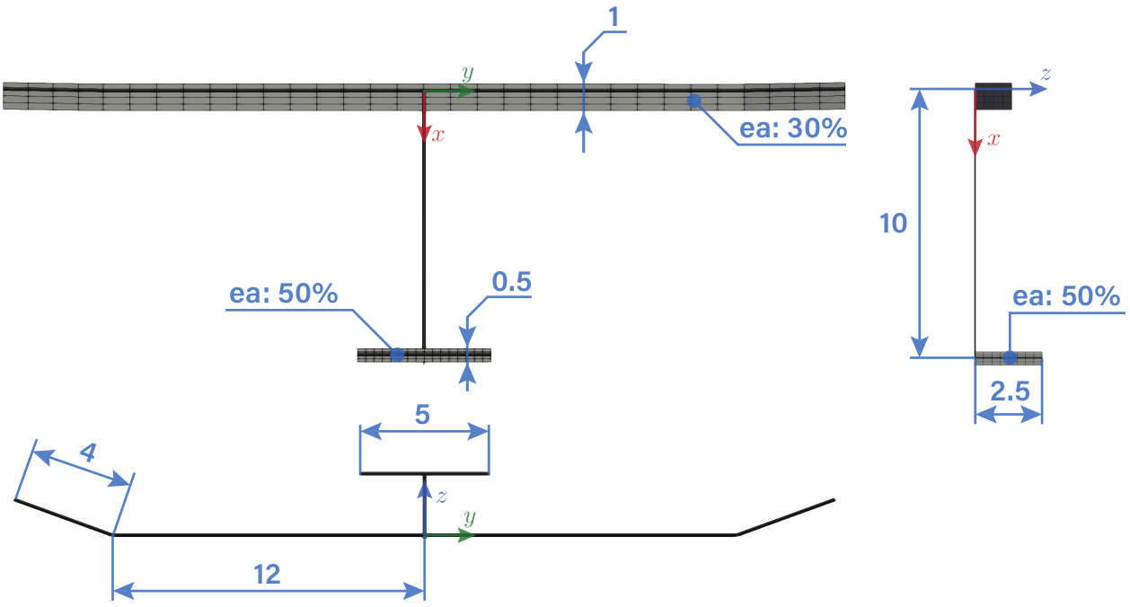
T-Tail HALE Model tutorial

The HALE T-Tail model intends to be a representative example of a typical HALE configuration, with high flexibility and aspect-ratio.

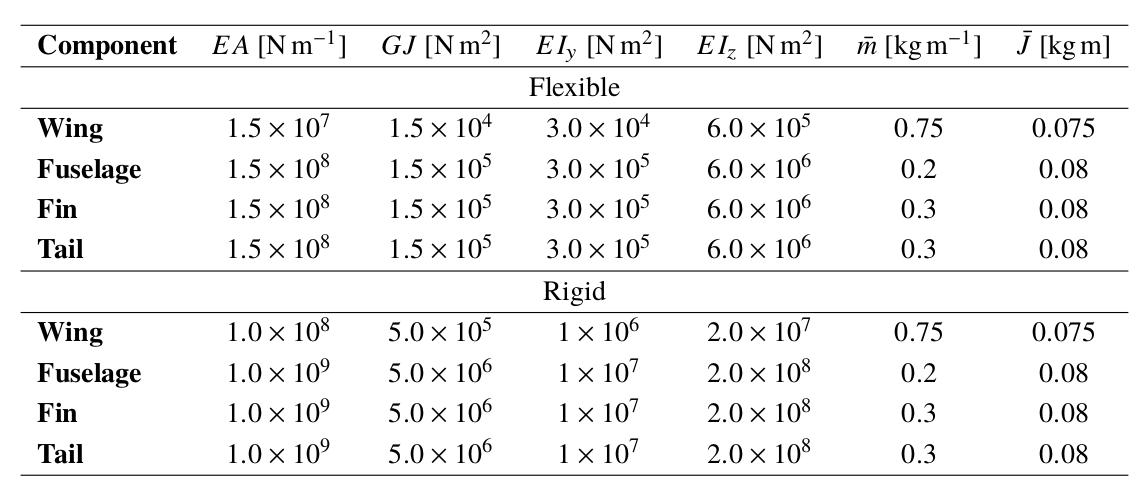
A geometry outline and a summary of the beam properties are given next

url = 'https://raw.githubusercontent.com/ImperialCollegeLondon/sharpy/dev_doc/docs/source/content/example_notebooks/images/t-tail_geometry.png'
Image(url=url, width=800)

url = 'https://raw.githubusercontent.com/ImperialCollegeLondon/sharpy/dev_doc/docs/source/content/example_notebooks/images/t-tail_properties.png'
Image(url=url, width=500)

This case is included in tests/coupled/simple_HALE/. The generate_hale.py file in that folder is the one that, if executed, generates all the required SHARPy files. This document is a step by step guide to how to process that case.

The T-Tail HALE model is subject to a 20% 1-cos spanwise constant gust.

First, let’s start with importing SHARPy in our Python environment.

import sharpy
import sharpy.sharpy_main as sharpy_main

And now the generate_HALE.py file needs to be executed.

route_to_case = '../../../../cases/coupled/simple_HALE/'
%run '../../../../cases/coupled/simple_HALE/generate_hale.py'

There should be 3 new files, apart from the original generate_hale.py:

!ls ../../../../cases/coupled/simple_HALE/

generate_hale.py  simple_HALE.aero.h5  simple_HALE.fem.h5  simple_HALE.sharpy

SHARPy can be run now. In the terminal, doing cd to the simple_HALE folder, the command would look like:

sharpy simple_HALE.sharpy

From a python console with import sharpy already run, the command is:

case_data = sharpy_main.main(['', route_to_case + 'simple_HALE.sharpy'])

/home/ad214/run/code_doc/sharpy/sharpy/aero/utils/uvlmlib.py:230: RuntimeWarning: invalid value encountered in true_divide
  flightconditions.uinf_direction = np.ctypeslib.as_ctypes(ts_info.u_ext[0][:, 0, 0]/flightconditions.uinf)
/home/ad214/run/code_doc/sharpy/sharpy/aero/utils/uvlmlib.py:347: RuntimeWarning: invalid value encountered in true_divide
  flightconditions.uinf_direction = np.ctypeslib.as_ctypes(ts_info.u_ext[0][:, 0, 0]/flightconditions.uinf)

The resulting data structure that is returned from the call to main contains all the time-dependant variables for both the structural and aerodynamic solvers.

timestep_info can be found in case_data.structure and case_data.aero. It is an array with custom-made structure to contain the data of each solver.

In the .sharpy file, we can see which solvers are run:

flow = ['BeamLoader',
        'AerogridLoader',
        'StaticTrim',
        'BeamLoads',
        'AerogridPlot',
        'BeamPlot',
        'DynamicCoupled',
        ]

In order:

• BeamLoader: reads the fem.h5 file and generates the structure for the beam solver.
• AerogridLoader: reads the aero.h5 file and generates the aerodynamic grid for the aerodynamic solver.
• StaticTrim: this solver performs a longitudinal trim (Thrust, Angle of attack and Elevator deflection) using the StaticCoupled solver.
• BeamLoads: calculates the internal beam loads for the static solution
• AerogridPlot: outputs the aerodynamic grid for the static solution.
• BeamPlot: outputs the structural discretisation for the static solution.
• DynamicCoupled: is the main driver of the dynamic simulation: executes the structural and aerodynamic solvers and couples both. Every converged time step is followed by a BeamLoads, AerogridPlot and BeamPlot execution.

Structural data organisation

The timestep_info structure contains several relevant variables:

• for_pos: position of the body-attached frame of reference in inertial FoR.
• for_vel: velocity (in body FoR) of the body FoR wrt inertial FoR.
• pos: nodal position in A FoR.
• psi: nodal rotations (from the material B FoR to A FoR) in a Cartesian Rotation Vector parametrisation.
• applied_steady_forces: nodal forces from the aero solver and the applied forces.
• postproc_cell: is a dictionary that contains the variables generated by a postprocessor, such as the internal beam loads.

The structural timestep_info also contains some useful variables:

• cag and cga return \(C^{AG}\) and \(C^{GA}\), the rotation matrices from the body-attached (A) FoR to the inertial (G).
• glob_pos rotates the pos variable to give you the inertial nodal position. If include_rbm = True is passed, for_pos is added to it.

Aerodynamic data organisation

The aerodynamic datastructure can be found in case_data.aero.timestep_info. It contains useful variables, such as:

• dimensions and dimensions_star: gives the dimensions of every surface and wake surface. Organised as: dimensions[i_surf, 0] = chordwise panels, dimensions[i_surf, 1] = spanwise panels.
• zeta and zeta_star: they are the \(G\) FoR coordinates of the surface vertices.
• gamma and gamma_star: vortex ring circulations.

Structural dynamics

We can now plot the rigid body dynamics:

RBM trajectory

fig, ax = plt.subplots(1, 1, figsize=(7, 4))

# extract information
n_tsteps = len(case_data.structure.timestep_info)
xz = np.zeros((n_tsteps, 2))
for it in range(n_tsteps):
    xz[it, 0] = -case_data.structure.timestep_info[it].for_pos[0] # the - is so that increasing time -> increasing x
    xz[it, 1] = case_data.structure.timestep_info[it].for_pos[2]
ax.plot(xz[:, 0], xz[:, 1])
fig.suptitle('Longitudinal trajectory of the T-Tail model in a 20% 1-cos gust encounter')
ax.set_xlabel('X [m]')
ax.set_ylabel('Z [m]');
plt.show()

RBM velocities

fig, ax = plt.subplots(3, 1, figsize=(7, 6), sharex=True)
ylabels = ['Vx [m/s]', 'Vy [m/s]', 'Vz [m/s]']

# extract information
n_tsteps = len(case_data.structure.timestep_info)
dt = case_data.settings['DynamicCoupled']['dt'].value
time_vec = np.linspace(0, n_tsteps*dt, n_tsteps)
for_vel = np.zeros((n_tsteps, 3))
for it in range(n_tsteps):
    for_vel[it, 0:3] = case_data.structure.timestep_info[it].for_vel[0:3]

for idim in range(3):
    ax[idim].plot(time_vec, for_vel[:, idim])
    ax[idim].set_ylabel(ylabels[idim])

ax[2].set_xlabel('time [s]')
plt.subplots_adjust(hspace=0)
fig.suptitle('Linear RBM velocities. T-Tail model in a 20% 1-cos gust encounter');
# ax.set_xlabel('X [m]')
# ax.set_ylabel('Z [m]');
plt.show()

fig, ax = plt.subplots(3, 1, figsize=(7, 6), sharex=True)
ylabels = ['Roll rate [deg/s]', 'Pitch rate [deg/s]', 'Yaw rate [deg/s]']

# extract information
n_tsteps = len(case_data.structure.timestep_info)
dt = case_data.settings['DynamicCoupled']['dt'].value
time_vec = np.linspace(0, n_tsteps*dt, n_tsteps)
for_vel = np.zeros((n_tsteps, 3))
for it in range(n_tsteps):
    for_vel[it, 0:3] = case_data.structure.timestep_info[it].for_vel[3:6]*180/np.pi

for idim in range(3):
    ax[idim].plot(time_vec, for_vel[:, idim])
    ax[idim].set_ylabel(ylabels[idim])

ax[2].set_xlabel('time [s]')
plt.subplots_adjust(hspace=0)
fig.suptitle('Angular RBM velocities. T-Tail model in a 20% 1-cos gust encounter');
# ax.set_xlabel('X [m]')
# ax.set_ylabel('Z [m]');
plt.show()

Wing tip deformation

It is stored in timestep_info as pos. We need to find the correct node.

fig, ax = plt.subplots(1, 1, figsize=(6, 6))
ax.scatter(case_data.structure.ini_info.pos[:, 0], case_data.structure.ini_info.pos[:, 1])
ax.axis('equal')
tip_node = np.argmax(case_data.structure.ini_info.pos[:, 1])
print('Wing tip node is the maximum Y one: ', tip_node)
ax.scatter(case_data.structure.ini_info.pos[tip_node, 0], case_data.structure.ini_info.pos[tip_node, 1], color='red')
plt.show()

Wing tip node is the maximum Y one:  16

We can plot now the pos[tip_node,:] variable:

fig, ax = plt.subplots(1, 1, figsize=(7, 3))

# extract information
n_tsteps = len(case_data.structure.timestep_info)
xz = np.zeros((n_tsteps, 2))
for it in range(n_tsteps):
    xz[it, 0] = case_data.structure.timestep_info[it].pos[tip_node, 0]
    xz[it, 1] = case_data.structure.timestep_info[it].pos[tip_node, 2]
ax.plot(time_vec, xz[:, 1])
# fig.suptitle('Longitudinal trajectory of the T-Tail model in a 20% 1-cos gust encounter')
ax.set_xlabel('time [s]')
ax.set_ylabel('Vertical disp. [m]');
plt.show()

fig, ax = plt.subplots(1, 1, figsize=(7, 3))

# extract information
n_tsteps = len(case_data.structure.timestep_info)
xz = np.zeros((n_tsteps, 2))
for it in range(n_tsteps):
    xz[it, 0] = case_data.structure.timestep_info[it].pos[tip_node, 0]
    xz[it, 1] = case_data.structure.timestep_info[it].pos[tip_node, 2]
ax.plot(time_vec, xz[:, 0])
# fig.suptitle('Longitudinal trajectory of the T-Tail model in a 20% 1-cos gust encounter')
ax.set_xlabel('time [s]')
ax.set_ylabel('Horizontal disp. [m]\nPositive is aft');
plt.show()

Wing root loads

The wing root loads can be extracted from the postproc_cell structure in timestep_info.

fig, ax = plt.subplots(3, 1, figsize=(7, 6), sharex=True)
ylabels = ['Torsion [Nm2]', 'OOP [Nm2]', 'IP [Nm2]']

# extract information
n_tsteps = len(case_data.structure.timestep_info)
dt = case_data.settings['DynamicCoupled']['dt'].value
time_vec = np.linspace(0, n_tsteps*dt, n_tsteps)
loads = np.zeros((n_tsteps, 3))
for it in range(n_tsteps):
    loads[it, 0:3] = case_data.structure.timestep_info[it].postproc_cell['loads'][0, 3:6]

for idim in range(3):
    ax[idim].plot(time_vec, loads[:, idim])
    ax[idim].set_ylabel(ylabels[idim])

ax[2].set_xlabel('time [s]')
plt.subplots_adjust(hspace=0)
fig.suptitle('Wing root loads. T-Tail model in a 20% 1-cos gust encounter');
# ax.set_xlabel('X [m]')
# ax.set_ylabel('Z [m]');
plt.show()

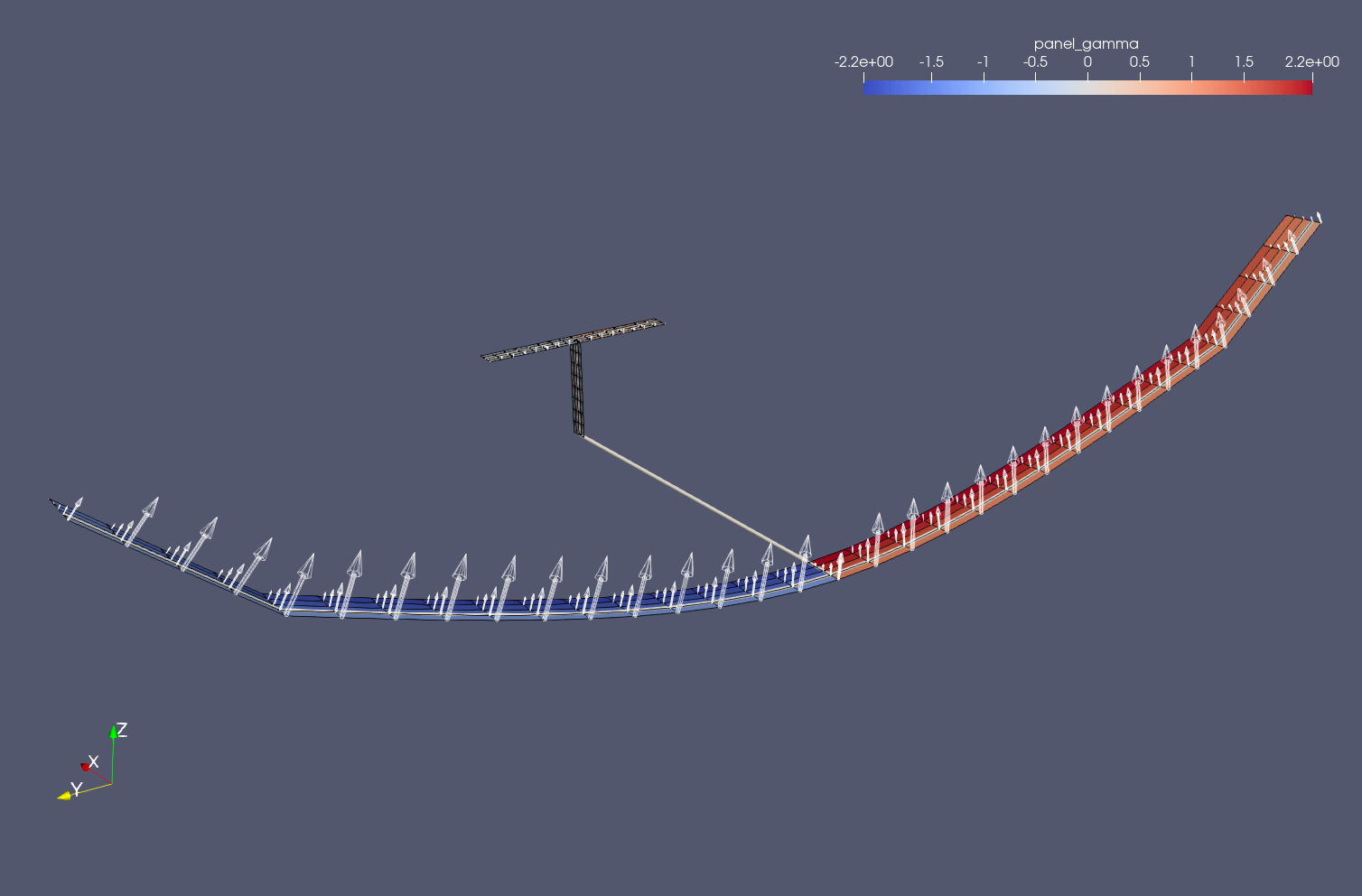
Aerodynamic analysis

The aerodynamic analysis can be obviously conducted using python. However, the easiest way is to run the case by yourself and open the files in output/simple_HALE/beam and output/simple_HALE/aero with Paraview.

url = 'https://raw.githubusercontent.com/ImperialCollegeLondon/sharpy/dev_doc/docs/source/content/example_notebooks/images/t-tail_solution.png'
Image(url=url, width=600)