Flutter Analysis of Goland’s Wing
Description
This is simple rectangular wing with constant properties originally proposed by Martin Goland in 1945 as a flutter benchmark case. This example generates a beam/UVLM model with the original properties in SHARPy and computes flutter around an arbitrary equilibrium point using the following general process:
Calculate steady aerodynamic forces and deflections for a given angle of attack using a nonlinear solver
Linearise the dynamic aeroelastic equations about this reference condition
Reduce the size of the (linearized) structural subsystem using modal projection
Reduce the size of the (linearized) aerodyanic subsystem using a Krylov projection
Evaluate the stability of the linearised aeroelastic system at different velocities and plot the results.
Wing properties
Span: b=20 ft., chord: c=6 ft., weight: 4 psi., radius of gyration about CG: .25c, elastic axis: 0.33c, centre of gravity: 0.43c
References
Goland, M. (1945). The Flutter o a Uniorm Cantilever Wing. Journal of Applied Mechanics,12(4):197-208.
Maraniello, S., & Palacios, R. (2019). State-Space Realizations and Internal Balancing in Potential-Flow Aerodynamics with Arbitrary Kinematics. AIAA Journal, 57(6):1–14. https://doi.org/10.2514/1.J058153
Latest update, RPN 14.05.2023
Required Packages
[1]:
import numpy as np
import matplotlib.pyplot as plt
import os
import sys
import sharpy.cases.templates.flying_wings as wings  # See this package for the Goland wing structural and aerodynamic definition
import sharpy.sharpy_main  # used to run SHARPy from Jupyter
Problem Set-up
Operatig conditions
The UVLM is assembled in normalised time at a velocity of \(1 m/s\). The only matrices that need updating then with free stream velocity are the structural matrices, which is significantly cheaper to do than to update the UVLM.
[2]:
u_inf = 1.
alpha_deg = 2.  # Define angle of attack for static aeroelastic analysis.
rho = 1.02      # Air density.
Discretisation
Note: To achieve convergence of the flutter results with the ones found in the literature, a fine grid is needed. If you are running this notebook for the first time, set M = 4 initially to verify that your system can perform!
[3]:
M = 16             # Number of chordwise panels
N = 32             # Number of spanwise panels
M_star_fact = 10   # Length of the wake in chords.
num_modes =  8     # Number of vibration modes retained in the structural model.
ROM
A moment-matching (Krylov subspace) model order reduction technique is employed. This ROM method offers the ability to interpolate the transfer functions at a desired point in the complex plane. See the ROM documentation pages for more info. Note that this ROM method matches the transfer function but does not guarantee stability. Therefore the resulting system may be unstable. These unstable modes may appear far in the right hand plane but will not affect the flutter speed calculations.
[4]:
c_ref = 1.8288 # Goland wing reference chord. Used for reduced frequency normalisation
rom_settings = dict()
rom_settings['algorithm'] = 'mimo_rational_arnoldi'  # reduction algorithm
rom_settings['r'] = 6  # Krylov subspace order
frequency_continuous_k = np.array([0.])  # Interpolation point in the complex plane with reduced frequency units
frequency_continuous_w = 2 * u_inf * frequency_continuous_k / c_ref
rom_settings['frequency'] = frequency_continuous_w
Case Admin
[5]:
case_name = 'goland_cs'
case_nlin_info = 'M%dN%dMs%d_nmodes%d' % (M, N, M_star_fact, num_modes)
case_rom_info = 'rom_MIMORA_r%d_sig%04d_%04dj' % (rom_settings['r'], frequency_continuous_k[-1].real * 100,
                                                  frequency_continuous_k[-1].imag * 100)

case_name += case_nlin_info + case_rom_info
route_test_dir = os.path.abspath('')

print('The case to run will be: %s' % case_name)
print('Case files will be saved in ./cases/%s' %case_name)
print('Output files will be saved in ./output/%s/' %case_name)
The case to run will be: goland_csM16N32Ms10_nmodes8rom_MIMORA_r6_sig0000_0000j
Case files will be saved in ./cases/goland_csM16N32Ms10_nmodes8rom_MIMORA_r6_sig0000_0000j
Output files will be saved in ./output/goland_csM16N32Ms10_nmodes8rom_MIMORA_r6_sig0000_0000j/
Simulation Set-Up
Goland Wing
ws is an instance of a Goland wing with a control surface. Reference the template file sharpy.cases.templates.flying_wings.GolandControlSurface for more info on the geometrical, structural and aerodynamic definition of the Goland wing here used.
[6]:
ws = wings.GolandControlSurface(M=M,
                                N=N,
                                Mstar_fact=M_star_fact,
                                u_inf=u_inf,
                                alpha=alpha_deg,
                                cs_deflection=[0, 0],
                                rho=rho,
                                sweep=0,
                                physical_time=2,
                                n_surfaces=2,
                                route=route_test_dir + '/cases',
                                case_name=case_name)

ws.clean_test_files()
ws.update_derived_params()
ws.set_default_config_dict()

ws.generate_aero_file()
ws.generate_fem_file()
Simulation Settings
The settings for each of the solvers are now set. For a detailed description on them please reference their respective documentation pages
SHARPy Settings
The most important setting is the flow list. It tells SHARPy which solvers to run and in which order.
[7]:
ws.config['SHARPy'] = {
    'flow':
        ['BeamLoader', 'AerogridLoader',
         'StaticCoupled',
         'AerogridPlot',
         'BeamPlot',
         'Modal',
         'LinearAssembler',
         'AsymptoticStability',
         ],
    'case': ws.case_name, 'route': ws.route,
    'write_screen': 'off', 'write_log': 'on',    # Change to 'on' as neded.
    'log_folder': route_test_dir + '/output/',
    'log_file': ws.case_name + '.log'}
Beam Loader Settings
[8]:
ws.config['BeamLoader'] = {
    'unsteady': 'off',
    'orientation': ws.quat}
Aerogrid Loader Settings
[9]:
ws.config['AerogridLoader'] = {
    'unsteady': 'off',
    'aligned_grid': 'on',
    'mstar': ws.Mstar_fact * ws.M,
    'freestream_dir': ws.u_inf_direction,
    'wake_shape_generator': 'StraightWake',
    'wake_shape_generator_input': {'u_inf': ws.u_inf,
                                    'u_inf_direction': ws.u_inf_direction,
                                    'dt': ws.dt}}
Static Coupled Solver
[10]:
ws.config['StaticCoupled'] = {
    'print_info': 'on',
    'max_iter': 200,
    'n_load_steps': 1,
    'tolerance': 1e-10,
    'relaxation_factor': 0.,
    'aero_solver': 'StaticUvlm',
    'aero_solver_settings': {
        'rho': ws.rho,
        'print_info': 'off',
        'horseshoe': 'off',
        'num_cores': 4,
        'n_rollup': 0,
        'rollup_dt': ws.dt,
        'rollup_aic_refresh': 1,
        'rollup_tolerance': 1e-4,
        'velocity_field_generator': 'SteadyVelocityField',
        'velocity_field_input': {
            'u_inf': ws.u_inf,
            'u_inf_direction': ws.u_inf_direction}},
    'structural_solver': 'NonLinearStatic',
    'structural_solver_settings': {'print_info': 'off',
                                   'max_iterations': 150,
                                   'num_load_steps': 4,
                                   'delta_curved': 1e-1,
                                   'min_delta': 1e-10,
                                   'gravity_on': 'on',
                                   'gravity': 9.81}}
AerogridPlot Settings
[11]:
ws.config['AerogridPlot'] = {'include_rbm': 'off',
                             'include_applied_forces': 'on',
                             'minus_m_star': 0}
BeamPlot Settings
[12]:
ws.config['BeamPlot'] = {'include_rbm': 'off',
                         'include_applied_forces': 'on'}
Modal Solver Settings
[13]:
ws.config['Modal'] = {'NumLambda': 20,
                      'rigid_body_modes': 'off',
                      'print_matrices': 'on', # 'keep_linear_matrices': 'on',            'write_dat': 'off',
                      'rigid_modes_cg': 'off',
                      'continuous_eigenvalues': 'off',
                      'dt': 0,
                      'plot_eigenvalues': False,
                      'max_rotation_deg': 15.,
                      'max_displacement': 0.15,
                      'write_modes_vtk': True,
                      'use_undamped_modes': True}
Linear System Assembly Settings
[14]:
ws.config['LinearAssembler'] = {'linear_system': 'LinearAeroelastic',
                                'linear_system_settings': {
                                    'beam_settings': {'modal_projection': 'on',
                                                      'inout_coords': 'modes',
                                                      'discrete_time': 'on',
                                                      'newmark_damp': 0.5e-4,
                                                      'discr_method': 'newmark',
                                                      'dt': ws.dt,
                                                      'proj_modes': 'undamped',
                                                      'use_euler': 'off',
                                                      'num_modes': num_modes,
                                                      'print_info': 'on',
                                                      'gravity': 'on',
                                                      'remove_sym_modes': 'on',
                                                      'remove_dofs': []},
                                    'aero_settings': {'dt': ws.dt,
                                                      'ScalingDict': {'length': 0.5 * ws.c_ref,
                                                                      'speed': u_inf,
                                                                      'density': rho},
                                                      'integr_order': 2,
                                                      'density': ws.rho,
                                                      'remove_predictor': 'on',
                                                      'use_sparse': 'on',
                                                      'remove_inputs': ['u_gust'],
                                                      'rom_method': ['Krylov'],
                                                      'rom_method_settings': {'Krylov': rom_settings}},
                                    }}
Asymptotic Stability Analysis Settings
[15]:
ws.config['AsymptoticStability'] = {'print_info': True,
                                    'velocity_analysis': [100, 180, 81],
                                   'modes_to_plot': []}
Write solver settings config file
[16]:
ws.config.write()
Run SHARPy
[17]:
sharpy.sharpy_main.main(['', ws.route + ws.case_name + '.sharpy'])
fatal: not a git repository (or any of the parent directories): .git
/home/rpalacio/anaconda3/envs/sharpy/lib/python3.10/site-packages/scipy/sparse/_index.py:146: SparseEfficiencyWarning: Changing the sparsity structure of a csc_matrix is expensive. lil_matrix is more efficient.
  self._set_arrayXarray(i, j, x)
/home/rpalacio/anaconda3/envs/sharpy/lib/python3.10/site-packages/sharpy/linear/src/lingebm.py:313: UserWarning: Euler parametrisation not implemented - Either rigid body modes are not being used or this method has already been called.
  warnings.warn('Euler parametrisation not implemented - Either rigid body modes are not being used or this '
/home/rpalacio/anaconda3/envs/sharpy/lib/python3.10/site-packages/sharpy/rom/krylov.py:242: UserWarning: Reduced Order Model Unstable
  warn.warn('Reduced Order Model Unstable')
[17]:
<sharpy.presharpy.presharpy.PreSharpy at 0x7f90aedb16c0>
Analysis
Nonlinear equilibrium
The nonlinear equilibrium condition can be visualised and analysed by opening, with Paraview, the files in the /output/<case_name>/aero and /output/<case_name>/beam folders to see the deflection and aerodynamic forces acting on the wing.
Stability
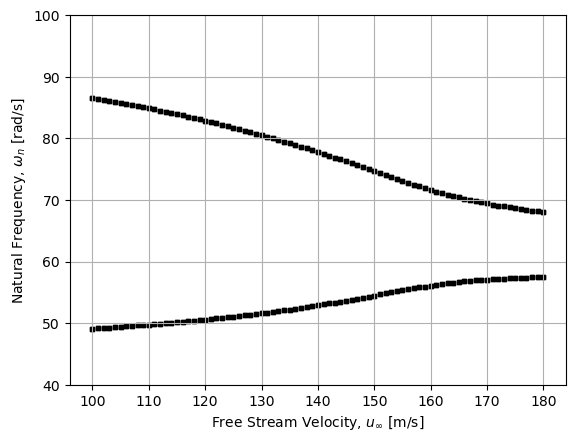
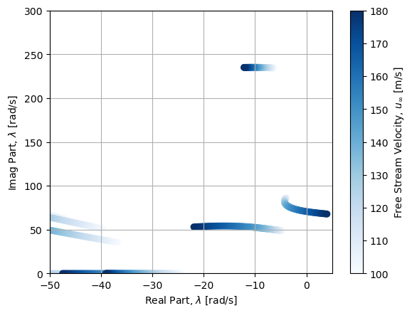
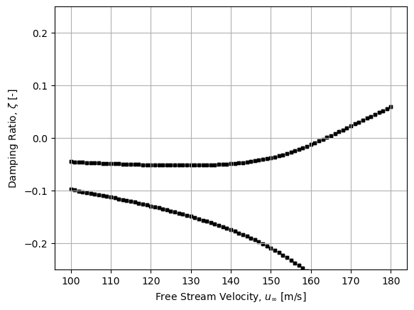
The stability of the Goland wing is now analysed under changing free stream velocity. The flutter modes involves the two lowest frequency modes near the imaginary axis (1st bending and 1st torsion if aerodynamics is removed). The two modes are seen quite separated at 100 m/s. As speed is increased, the damping of the torsion mode decreases until it crosses the imaginary axis onto the right hand plane and flutter begins.
[18]:
file_name = './output/%s/stability/velocity_analysis_min1000_max1800_nvel0081.dat' % case_name

velocity_analysis = np.loadtxt(file_name)
u_inf = velocity_analysis[:, 0]
eigs_r = velocity_analysis[:, 1]
eigs_i = velocity_analysis[:, 2]
[23]:
fig = plt.figure()
plt.scatter(eigs_r, eigs_i, c=u_inf, cmap='Blues')
cbar = plt.colorbar()
cbar.set_label('Free Stream Velocity, $u_\infty$ [m/s]')

plt.grid()
plt.xlim(-50, 5)
plt.ylim(0, 300)
plt.xlabel('Real Part, $\lambda$ [rad/s]')
plt.ylabel('Imag Part, $\lambda$ [rad/s]');
[20]:
fig = plt.figure()
natural_frequency = np.sqrt(eigs_r ** 2 + eigs_i ** 2)
damping_ratio = eigs_r / natural_frequency
cond = (eigs_r>-25) * (eigs_r<10) * (natural_frequency<100) # filter unwanted eigenvalues for this plot (mostly aero modes)

plt.scatter(u_inf[cond], damping_ratio[cond], color='k', marker='s', s=9)

plt.grid()
plt.ylim(-0.25, 0.25)
plt.xlabel('Free Stream Velocity, $u_\infty$ [m/s]')
plt.ylabel('Damping Ratio, $\zeta$ [-]');
[21]:
fig = plt.figure()
cond = (eigs_r>-25) * (eigs_r<10) # filter unwanted eigenvalues for this plot (mostly aero modes)
plt.scatter(u_inf[cond], natural_frequency[cond], color='k', marker='s', s=9)

plt.grid()
plt.ylim(40, 100)
plt.xlabel('Free Stream Velocity, $u_\infty$ [m/s]')
plt.ylabel('Natural Frequency, $\omega_n$ [rad/s]');